03 - Kaiser-Squires: Physics and Practice

Learning Objectives

By the end of this tutorial, you should be able to:

1. Explain what the Kaiser-Squires (KS) inversion is reconstructing physically.

2. Connect core KS assumptions to practical analysis choices in SMPy.

3. Run KS in SMPy and interpret E/B maps, including smoothing tradeoffs.

Canonical Reference

The foundational paper for this method is:

• Kaiser, N. & Squires, G. (1993), Mapping the dark matter with weak gravitational lensing, The Astrophysical Journal, 404, 441-450. DOI: 10.1086/172297 ADS: 1993ApJ…404..441K

1) Physics Primer

Weak lensing maps how light from background galaxies is distorted by foreground mass.

The local lensing distortion is described by the Jacobian

\[\begin{split}\mathbf{A}(\boldsymbol{\theta}) = \begin{pmatrix} 1-\kappa-\gamma_1 & -\gamma_2 \\ -\gamma_2 & 1-\kappa+\gamma_1 \end{pmatrix}\end{split}\]

where:

• \(\kappa\): convergence (projected surface-density contrast)

• \(\gamma_1, \gamma_2\): shear components

Observed galaxy shapes estimate the reduced shear:

\[\mathbf{g} = \frac{\boldsymbol{\gamma}}{1-\kappa}\]

In the weak regime (\(|\kappa| \ll 1\)), we often use \(\mathbf{g} \approx \boldsymbol{\gamma}\).

2) KS Inversion in Fourier Space

Define complex shear and convergence:

\[\gamma = \gamma_1 + i\gamma_2, \qquad \kappa = \kappa_E + i\kappa_B\]

Kaiser-Squires uses the Fourier-space relation

\[\hat{\gamma}(\boldsymbol{\ell}) = D(\boldsymbol{\ell})\,\hat{\kappa}(\boldsymbol{\ell}), \qquad D(\boldsymbol{\ell}) = \frac{\ell_1^2 - \ell_2^2 + 2i\ell_1\ell_2}{\ell_1^2 + \ell_2^2}\]

So the inversion is

\[\hat{\kappa}(\boldsymbol{\ell}) = D^*(\boldsymbol{\ell})\,\hat{\gamma}(\boldsymbol{\ell})\]

The real part gives E-mode convergence (physical lensing signal), while the imaginary part gives B-mode (often used as a systematics diagnostic).

3) Practical Assumptions and Caveats

Important assumptions behind basic KS usage:

• Flat-sky approximation (appropriate for modest fields of view).

• Finite survey boundaries can leak power and bias edges.

• Smoothing reduces noise but also suppresses small-scale structure.

• Mass-sheet degeneracy remains a fundamental lensing ambiguity.

This is why diagnostics (especially B-mode behavior and sensitivity to smoothing) are part of good practice.

4) Mapping Physics to SMPy Settings

In SMPy, the main KS-relevant controls are:

• general.coordinate_system: radec or pixel

• general.radec.resolution (or API pixel_scale): angular map resolution

• methods.kaiser_squires.smoothing.sigma (or API smoothing): Gaussian smoothing scale

• general.mode: ['E'], ['B'], or ['E', 'B']

For this tutorial we will run in radec, produce both E and B maps, and compare multiple smoothing values.

5) SMPy Analysis Workflow

A standard analysis workflow in SMPy is:

1. Set data paths and shear/coordinate column names.

2. Build a Config from method defaults and update the run parameters.

3. Save the config for provenance, then execute run(config).

4. Inspect E/B outputs and iterate on smoothing and diagnostics.

from pathlib import Path
import random

import numpy as np
import pandas as pd
import smpy
from IPython.display import Image, display

from smpy.config import Config
from smpy.run import run

# Set deterministic seeds for reproducible tutorial outputs.
SEED = 42
random.seed(SEED)
np.random.seed(SEED)


def find_repo_root(start: Path) -> Path:
    # Walk upward until we find the SMPy repository root markers.
    for candidate in [start, *start.parents]:
        if (candidate / "setup.py").exists() and (candidate / "smpy").is_dir():
            return candidate
    raise RuntimeError("Could not locate SMPy repository root.")


# Resolve input/output locations relative to the repository root.
repo_root = find_repo_root(Path.cwd().resolve())
data_file = repo_root / "examples" / "data" / "forecast_lum_annular.fits"
artifacts_dir = repo_root / "examples" / "outputs" / "tutorials"
artifacts_dir.mkdir(parents=True, exist_ok=True)

# Print runtime context for quick verification in notebook output.
print(f"SMPy version: {smpy.__version__}")
print(f"Seed: {SEED}")
print(f"Input data: {data_file}")
print(f"Output root: {artifacts_dir}")

SMPy version: 0.5.0
Seed: 42
Input data: /home/docs/checkouts/readthedocs.org/user_builds/smpy-docs/checkouts/latest/examples/data/forecast_lum_annular.fits
Output root: /home/docs/checkouts/readthedocs.org/user_builds/smpy-docs/checkouts/latest/examples/outputs/tutorials

base_name = "tutorial03_ks_workflow"

workflow_config = Config.from_defaults("kaiser_squires")
workflow_config.update_from_kwargs(
    data=str(data_file),
    coord_system="radec",
    pixel_scale=0.4,
    smoothing=2.0,
    g1_col="g1_Rinv",
    g2_col="g2_Rinv",
    weight_col="weight",
    mode=["E", "B"],
    save_plots=True,
    save_fits=False,
    output_dir=str(artifacts_dir),
    output_base_name=base_name,
)

workflow_config_path = artifacts_dir / "tutorial03_ks_workflow.yaml"
workflow_config.save_config(workflow_config_path)

result = run(workflow_config)

print("KS workflow run complete.")
print("E map shape:", result["maps"]["E"].shape)
print("B map shape:", result["maps"]["B"].shape)
print("E std:", float(np.nanstd(result["maps"]["E"])))
print("B std:", float(np.nanstd(result["maps"]["B"])))
print("Saved config snapshot:", workflow_config_path)

Configuration saved to: /home/docs/checkouts/readthedocs.org/user_builds/smpy-docs/checkouts/latest/examples/outputs/tutorials/tutorial03_ks_workflow.yaml
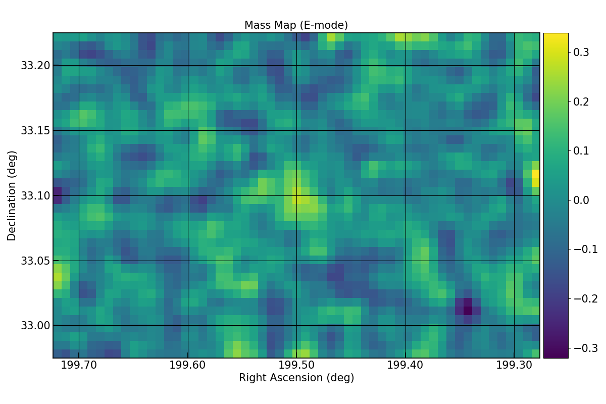
Convergence map saved as PNG file: /home/docs/checkouts/readthedocs.org/user_builds/smpy-docs/checkouts/latest/examples/outputs/tutorials/kaiser_squires/tutorial03_ks_workflow_kaiser_squires_e_mode.png
Convergence map saved as PNG file: /home/docs/checkouts/readthedocs.org/user_builds/smpy-docs/checkouts/latest/examples/outputs/tutorials/kaiser_squires/tutorial03_ks_workflow_kaiser_squires_b_mode.png
KS workflow run complete.
E map shape: (38, 57)
B map shape: (38, 57)
E std: 0.042875682598267024
B std: 0.03868921282648928
Saved config snapshot: /home/docs/checkouts/readthedocs.org/user_builds/smpy-docs/checkouts/latest/examples/outputs/tutorials/tutorial03_ks_workflow.yaml

ks_dir = artifacts_dir / "kaiser_squires"
baseline_e_png = ks_dir / f"{base_name}_kaiser_squires_e_mode.png"
baseline_b_png = ks_dir / f"{base_name}_kaiser_squires_b_mode.png"

print("Baseline SMPy plot outputs:")
print("-", baseline_e_png)
print("-", baseline_b_png)

if baseline_e_png.exists() and baseline_b_png.exists():
    display(Image(filename=str(baseline_e_png)))
    display(Image(filename=str(baseline_b_png)))
else:
    print("Expected PNG outputs were not found. Re-run the previous cell.")

Baseline SMPy plot outputs:
- /home/docs/checkouts/readthedocs.org/user_builds/smpy-docs/checkouts/latest/examples/outputs/tutorials/kaiser_squires/tutorial03_ks_workflow_kaiser_squires_e_mode.png
- /home/docs/checkouts/readthedocs.org/user_builds/smpy-docs/checkouts/latest/examples/outputs/tutorials/kaiser_squires/tutorial03_ks_workflow_kaiser_squires_b_mode.png

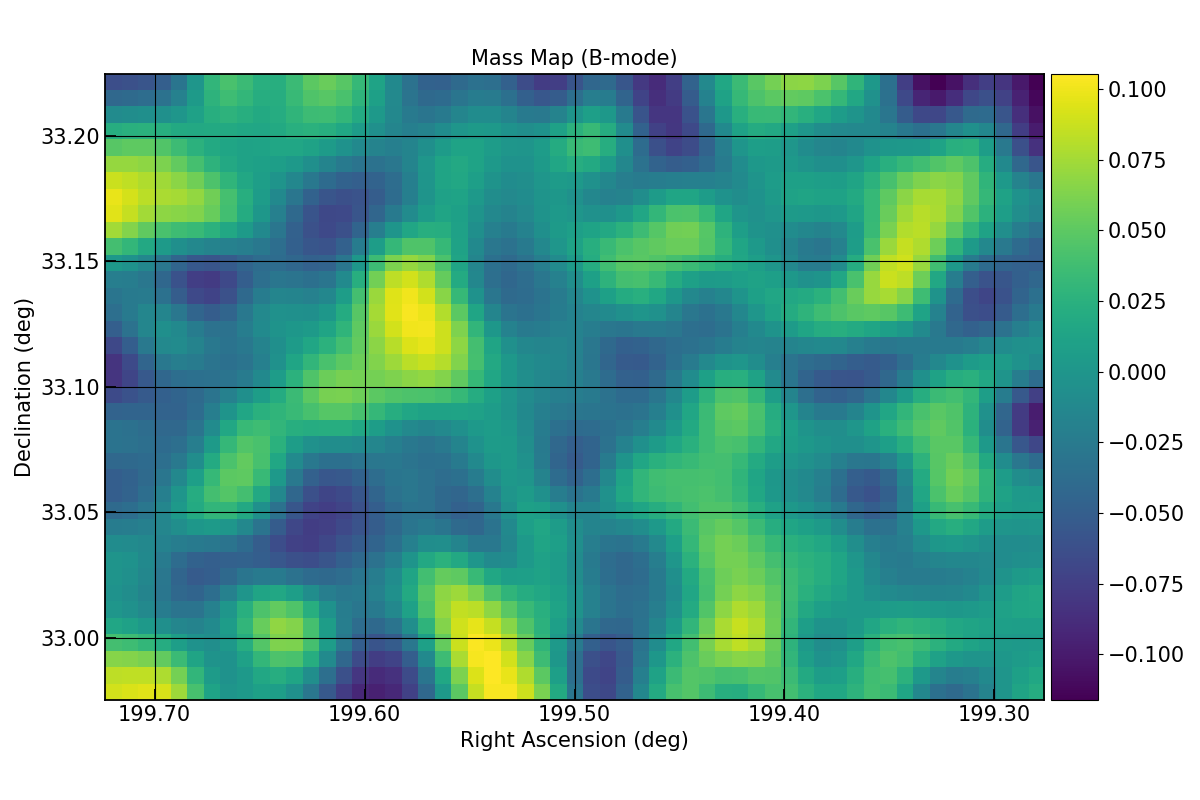
Interpretation (Baseline)

• The E-mode map is your primary mass-reconstruction product.

• The B-mode should generally be weaker and less spatially coherent than E-mode.

• A B-mode of similar strength/structure to E-mode is a warning sign to investigate systematics.

For parameter studies, the next section uses the Config API to run a controlled smoothing sweep.

smoothing_values = [1.0, 2.0, 4.0]
rows = []
run_records = []

for sigma in smoothing_values:
    sigma_tag = str(sigma).replace(".", "p")
    run_name = f"tutorial03_ks_sigma{sigma_tag}"

    cfg = Config.from_defaults("kaiser_squires")
    cfg.update_from_kwargs(
        data=str(data_file),
        coord_system="radec",
        pixel_scale=0.4,
        smoothing=sigma,
        g1_col="g1_Rinv",
        g2_col="g2_Rinv",
        weight_col="weight",
        mode=["E", "B"],
        save_plots=True,
        save_fits=False,
        output_dir=str(artifacts_dir),
        output_base_name=run_name,
    )

    cfg.validate()
    res = run(cfg)

    e_map = res["maps"]["E"]
    b_map = res["maps"]["B"]

    rows.append(
        {
            "smoothing_sigma": sigma,
            "E_std": float(np.nanstd(e_map)),
            "B_std": float(np.nanstd(b_map)),
            "E_max_abs": float(np.nanmax(np.abs(e_map))),
            "B_max_abs": float(np.nanmax(np.abs(b_map))),
            "B_to_E_std_ratio": float(np.nanstd(b_map) / np.nanstd(e_map)),
        }
    )

    run_records.append(
        {
            "sigma": sigma,
            "run_name": run_name,
            "e_png": ks_dir / f"{run_name}_kaiser_squires_e_mode.png",
            "b_png": ks_dir / f"{run_name}_kaiser_squires_b_mode.png",
        }
    )

summary = pd.DataFrame(rows).sort_values("smoothing_sigma")
summary_path = artifacts_dir / "ks_smoothing_summary.csv"
summary.to_csv(summary_path, index=False)

print(f"Saved summary table: {summary_path}")
summary

Convergence map saved as PNG file: /home/docs/checkouts/readthedocs.org/user_builds/smpy-docs/checkouts/latest/examples/outputs/tutorials/kaiser_squires/tutorial03_ks_sigma1p0_kaiser_squires_e_mode.png
Convergence map saved as PNG file: /home/docs/checkouts/readthedocs.org/user_builds/smpy-docs/checkouts/latest/examples/outputs/tutorials/kaiser_squires/tutorial03_ks_sigma1p0_kaiser_squires_b_mode.png
Convergence map saved as PNG file: /home/docs/checkouts/readthedocs.org/user_builds/smpy-docs/checkouts/latest/examples/outputs/tutorials/kaiser_squires/tutorial03_ks_sigma2p0_kaiser_squires_e_mode.png
Convergence map saved as PNG file: /home/docs/checkouts/readthedocs.org/user_builds/smpy-docs/checkouts/latest/examples/outputs/tutorials/kaiser_squires/tutorial03_ks_sigma2p0_kaiser_squires_b_mode.png
Convergence map saved as PNG file: /home/docs/checkouts/readthedocs.org/user_builds/smpy-docs/checkouts/latest/examples/outputs/tutorials/kaiser_squires/tutorial03_ks_sigma4p0_kaiser_squires_e_mode.png
Convergence map saved as PNG file: /home/docs/checkouts/readthedocs.org/user_builds/smpy-docs/checkouts/latest/examples/outputs/tutorials/kaiser_squires/tutorial03_ks_sigma4p0_kaiser_squires_b_mode.png
Saved summary table: /home/docs/checkouts/readthedocs.org/user_builds/smpy-docs/checkouts/latest/examples/outputs/tutorials/ks_smoothing_summary.csv

	smoothing_sigma	E_std	B_std	E_max_abs	B_max_abs	B_to_E_std_ratio
0	1.0	0.079732	0.079208	0.339032	0.287085	0.993431
1	2.0	0.042876	0.038689	0.165443	0.116255	0.902358
2	4.0	0.021592	0.016111	0.069374	0.061914	0.746153

print("E-mode outputs across smoothing values:")
for record in run_records:
    print(f"sigma={record['sigma']}: {record['e_png']}")
    if record["e_png"].exists():
        display(Image(filename=str(record["e_png"])))
    else:
        print("  Missing file; rerun smoothing cell above.")

E-mode outputs across smoothing values:
sigma=1.0: /home/docs/checkouts/readthedocs.org/user_builds/smpy-docs/checkouts/latest/examples/outputs/tutorials/kaiser_squires/tutorial03_ks_sigma1p0_kaiser_squires_e_mode.png

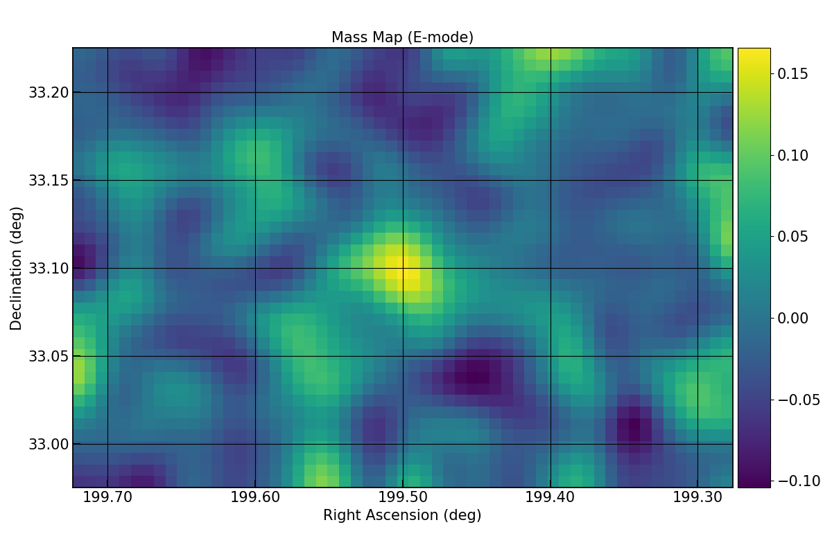
sigma=2.0: /home/docs/checkouts/readthedocs.org/user_builds/smpy-docs/checkouts/latest/examples/outputs/tutorials/kaiser_squires/tutorial03_ks_sigma2p0_kaiser_squires_e_mode.png

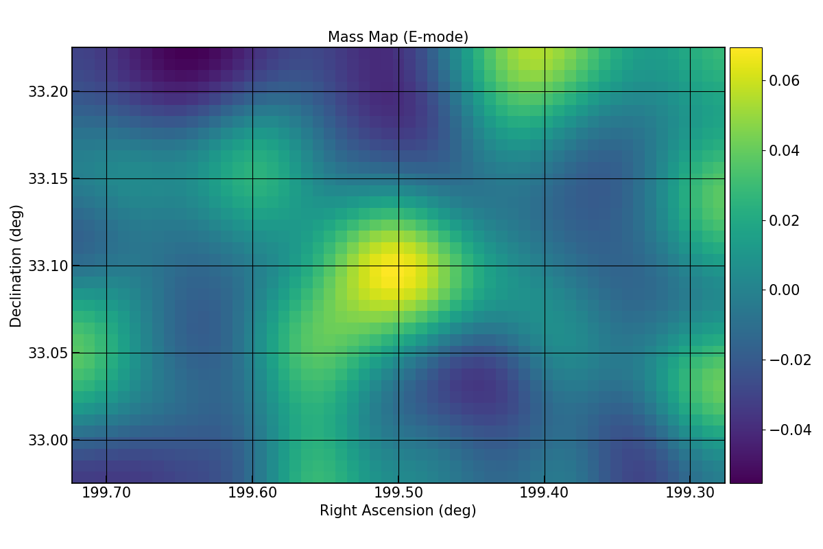
sigma=4.0: /home/docs/checkouts/readthedocs.org/user_builds/smpy-docs/checkouts/latest/examples/outputs/tutorials/kaiser_squires/tutorial03_ks_sigma4p0_kaiser_squires_e_mode.png

References

• Kaiser, N. & Squires, G. (1993), The Astrophysical Journal, 404, 441-450. DOI: 10.1086/172297

• ADS entry: 1993ApJ…404..441K